
Finance Help: Consider the mixed streams of cash flows shown in the following table
saxi753
Present value: Mixed streams Consider the mixed streams of cash flows shown in the following table
a. Find the present value of each stream using a 6% discount rate.
b. Compare the calculated present values and discuss them in light of the undiscounted cash flows totaling $70 comma 000 in each case. Is there some discount rate at which the present values of the two streams would be equal?
#FInanceHelp
#AccountingHelp
#Excel
#FutureValue
#Investments
Finance Help: Value of a mixed stream Harte Systems, Inc., a maker of electronic survillance
saxi753
Value of a mixed stream Harte Systems, Inc., a maker of electronic survillance equipment, is considering selling the rights to market its home security system to a well-known hardware chain. The proposed deal calls for the hardware chain to pay Harte $32000 and $25 000 at the end of years 1 and 2 and to make annual year-end payments of $12 000 in years 3 through 9. A final payment to Harte of $20 000 would be due at the end of year 10.
a. Select the time line that represents the cash flows involved in the offer.
b. If Harte applies a required rate of return of 9% to them, what is the present value of this series of payments?
c. A second company has offered Harte an immediate one-time payment of $110 000 for the rights to market the home security system. Which offer should Harte accept?
#FinanceHelp
#Excel
#AccountingHelp
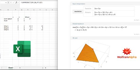
Toán Tối Ưu Hóa - Tìm kết quả tối ưu hóa bằng phần mềm Excel và WolframAlpha để kiểm tra -2 lựa chọn
saxi753
Đây là video cách giải chi tiết từng bước một về cách sử dụng phần mềm để tìm Tối Ưu Hóa (Không có trong sách giáo khoa Toán hiện tại)
#MicrosoftExcel
#WolframAlpha
#CachGiai
#Optimization
#Functions
#Inequality
#BatPhuongTrinh
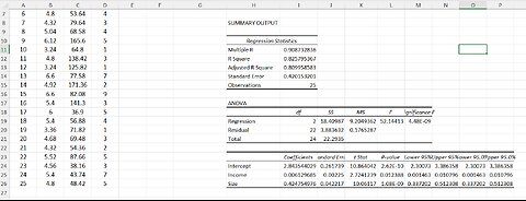
Excel Practice: How to make the Summary Output from the Data Analysis
saxi753
Many regions in North and South Carolina and Georgia have experienced rapid population growth over the last 10 years. It is expected that the growth will continue over the next 10 years. This has motivated many of the large grocery store chains to build new stores in the region. The Kelley's Super Grocery Stores Inc. chain is no exception. The director of planning for Kelley's Super Grocery Stores wants to study adding more stores in this region. He believes there are two main factors that indicate the amount families spend on groceries. The first is their income and the other is the number of people in the family. The director gathered the following sample information
#Excel
#Regression
#DataAnalysis

Diaz Marketing - SAM Project 1b Excel Module 01 Creating a Worksheet and a Chart - Step-by-step
saxi753
Shelly Cashman Excel 365/2021 | Module 1: SAM Project 1b
Diaz Marketing
COMPLETE A BUDGET SUMMARY WORKSHEET
GETTING STARTED
• Save the file SC_EX365_2021_1b_FirstLastName_1.xlsx as SC_EX365_2021_1b_FirstLastName_2.xlsx
o Edit the file name by changing “1” to “2”.
o If you do not see the .xlsx file extension, do not type it. The file extension will be added for you automatically.
• With the file SC_EX365_2021_1b_FirstLastName_2.xlsx open, ensure that your first and last name is displayed in cell B6 of the Documentation worksheet.
o If cell B6 does not display your name, delete the file and download a new copy.
PROJECT STEPS
1. Ashley Bowman manages the New England office for Diaz Marketing, a consulting firm that develops strategies for businesses to become more profitable. She has created a worksheet summarizing the revenue and expenses for the first six months of the year, and asks for your help in determining what the New England office needs to do in the rest of the year to meet its profit goals.
Go to the Budget worksheet. Cut the worksheet subtitle from cell B1 and paste it in cell A2 to display the subtitle in its expected location.
2. In cell H2, add the text consultants so that the complete text appears as "Number of consultants" and more clearly identifies the value in cell J2.
3. Enter Feb in cell C3, Mar in cell D3, Apr in cell E3, May in cell F3, and Jun in cell G3.
4. In cell J4, enter a formula that subtracts the value in cell I4 from the value in cell H4 to determine how much revenue the New England office needs to earn from July to December to reach its goal for the year.
5. Ashley wants to calculate the gross margin from January to June and for the year to date. Provide this information as follows:
a. In cell B6, enter a formula that divides the value in cell B5 (the gross profit for January) by the value in cell B4 (the revenue in January).
b. Use the Fill Handle to fill the range C6:H6 with the formula in cell B6 to find the gross margin for February to June and for the year to date.
6. Ashley needs to sum the sales for each New England state for the year to date. Provide this information as follows:
a. In cell H9, enter a formula that uses the SUM function to total the range B9:G9 to calculate the year-to-date sales for Connecticut.
b. Use the Fill Handle to fill the range H10:H12 with the formula in cell H9 to find the year-to-date sales for the other states.
7. In cell B17, enter 27,363 as the general expenses for January.
8. Ashley wants to determine how much revenue each state needs to generate from July to December to reach its target for the year. Enter this information as follows:
a. In cell J9, enter a formula that subtracts the value in cell I9 from the value in cell H9 to find the amount of Connecticut sales Ashley needs to meet the goal.
b. Copy the formula in cell J9, and then paste it in the range J10:J14, pasting the formulas only, to find the differences for the other states, the total, and the revenue per consultant.
9. Ashley is interested in how much revenue the nine consultants each generate on average per month and for the year to date. Find this information as follows:
a. Edit cell B14 to include a formula that divides the value in cell B13 (the total sales for Connecticut in January) by the value in cell J2 (the number of consultants). Don't change the reference to cell J2 that is already there.
b. Fill the range C14:H14 with the formula in cell B14 to determine the average revenue per consultant from February to June and for the year to date.
10. Ashley also needs to calculate the operating margin, which is the ratio of operating profit or loss to revenue and indicates how much the office makes after paying for expenses. Calculate the operating margin as follows:
a. In cell B19, enter a formula that divides the value in cell B18 (the operating profit or loss in January) by the value in cell B4 (the revenue in January).
b. Use the Fill Handle to fill the range C19:H19 with the formula in cell B19 to find the operating margin for February to June and for the year to date.
11. Ashley wants to visualize the total year to date sales separated into states. Insert a chart to provide this visualization as follows:
a. Create a 2-D Pie Chart based on the nonadjacent ranges A8:A12 and H8:H12.
b. Enter Total Year to Date Sales by State as the chart title.
c. Reposition and resize the chart so its upper-left corner is in cell K3 and its bottom-right corner is in cell M17
d. Apply Style 11 to the chart.
12. Hide the gridlines for the Budget worksheet to make it easier to read.
Your workbook should look like the Final Figures on the following pages. Save your changes, close the workbook, and then exit Excel. Follow the directions on the website to submit your completed project.
Final Figure 1: Budget Worksheet
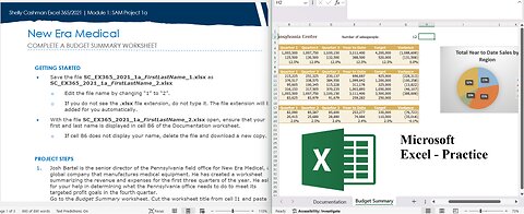
SAM Project 1a Excel Module 01 Creating a Worksheet and a Chart - New Era Medical COMPLETE A BUDGET
saxi753
Shelly Cashman Excel 365/2021 | Module 1: SAM Project 1a
New Era Medical
COMPLETE A BUDGET SUMMARY WORKSHEET
GETTING STARTED
• Save the file SC_EX365_2021_1a_FirstLastName_1.xlsx as SC_EX365_2021_1a_FirstLastName_2.xlsx
o Edit the file name by changing “1” to “2”.
o If you do not see the .xlsx file extension, do not type it. The file extension will be added for you automatically.
• With the file SC_EX365_2021_1a_FirstLastName_2.xlsx open, ensure that your first and last name is displayed in cell B6 of the Documentation worksheet.
o If cell B6 does not display your name, delete the file and download a new copy.
PROJECT STEPS
1. Josh Bartel is the senior director of the Pennsylvania field office for New Era Medical, a global company that manufactures medical equipment. He has created a worksheet summarizing the revenue and expenses for the first three quarters of the year. He asks for your help in determining what the Pennsylvania office needs to do to meet its targeted profit goals in the fourth quarter.
Go to the Budget Summary worksheet. Cut the worksheet title from cell I1 and paste it in cell A1 to display the title in its expected location.
2. In cell E2, add the text Number of so that the complete text appears as "Number of salespeople:" and more clearly identifies the value in cell G2.
3. Enter Quarter 2 in cell C4 and Quarter 3 in cell D4.
4. In cell G5, enter a formula without a function that subtracts the target revenue (cell F5) from the year to date revenue (cell E5) to determine how much revenue the field office needs to earn in Quarter 4 to reach its target for the year.
5. Josh wants to calculate the gross margin for Quarters 1–3 and the year to date. Provide this information as follows:
a. In cell B7, enter a formula without a function that divides the gross profit for Quarter 1 (cell B6) by the revenue in Quarter 1 (cell B5).
b. Fill the range C7:E7 with the formula in cell B7 to find the gross margin for Quarters 2 and 3 and for the year to date.
6. Josh needs to sum the sales for each Pennsylvania region for the year to date. Provide this information as follows:
a. In cell E10, enter a formula that uses the SUM function to total the regional sales data for the Northeast region (the range B10:D10) to calculate the year-to-date sales.
b. Use the Fill Handle to fill the range E11:E13 with the formula in cell E10 to find the year-to-date sales for the other three regions.
7. In cell F10, enter the value 925000 to provide the targeted annual sales amount for the Northeast region.
8. Josh wants to determine how much revenue each region needs to generate in Quarter 4 to reach its target for the year. Enter this information as follows:
a. In cell G10, enter a formula without a function that subtracts the target sales for the Northeast region (cell F10) from its year to date regional sales (cell E10) to find the amount of sales the Northeast region needs to generate to meet its target.
b. Copy the formula in cell G10, and then paste it in the range G11:G14, pasting the formulas only, to find the variances for the other regions and for the total.
9. Josh is interested in how much revenue each of the 12 salespeople generates on average in each quarter and for the year to date. Find this information as follows:
a. Edit cell B15 to include a formula without a function that divides the total regional sales in Quarter 1 (cell B14) by the number of salespeople (cell G2). Don't change the reference to cell G2 that is already there.
b. Fill the range C15:E15 with the formula in cell B15 to determine the average revenue per salesperson in Quarters 2 and 3 and for the year to date.
10. Josh also needs to calculate the operating margin, which is the ratio of operating profit or loss to revenue and indicates how much the office makes after paying for expenses. Calculate the operating margin as follows:
a. In cell B20, enter a formula without a function that divides the operating profit or loss in Quarter 1 (cell B19) by the revenue from Quarter 1 (cell B5).
b. Use the Fill Handle to fill the range C20:E20 with the formula in cell B20 to find the operating margin for Quarters 2 and 3 and for the year to date.
11. Josh wants to include a visualization of the total year to date sales separated by region. Insert a chart to provide this visualization as follows:
a. Create a 2-D Pie Chart based on the nonadjacent ranges A9:A13 and E9:E13.
b. Enter Total Year to Date Sales by Region as the chart title.
c. Resize and reposition the chart so its upper-left corner is in cell I4 and its bottom-right corner is in cell L18.
d. Apply Style 3 to the chart.
12. Hide the gridlines for the Budget Summary worksheet to make it easier to read.
Your workbook should look like the Final Figures on the following pages. Save your changes, close the workbook, and then exit Excel. Follow the directions on the website to submit your completed project.
Final Figure 1: Budget Summary Worksheet
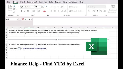
Finance Help: Suppose a 10-year, $1000 bond with a coupon rate of 9% and semiannual coupons is trade
saxi753
Finance Help: Suppose a 10-year, $1000 bond with a coupon rate of 9% and semiannual coupons is trade
#Excel
#MicrosoftExcel
#FinanceHelp
#Finance
#YeildToMaturity
#InterestRates
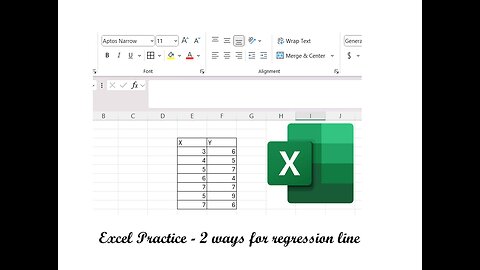
Excel: Two ways to make Regression Line on Microsoft Excel - Step-by-step
saxi753
Here is the technique to solve the question related to regression line and how to find them in step-by-step
#RegressionLine
#MicrosoftExcel
#Excel
#Table

Excel Practice: High-Low Method and Regression Line for Data Analysis/Accounting
saxi753
Here is the full video to show the step-by-step to do regression line and high-low method on Excel with step-by-step
#High-lowMethod
#RegressionLine
#Excel
#Techniques

Excel Practice: How to copy the database from Comparative Competitive Effort to Excel? BSG Mastery
saxi753
Here is the manual way to copy the database from Comparative Competitive Effort from BSG (Business Strategy Game) to Excel for analyzing, calculating, and making the other charts from Microsoft Excel
#MicrosoftExcel
#Excel
#Business
#Database
#DataAnalysis
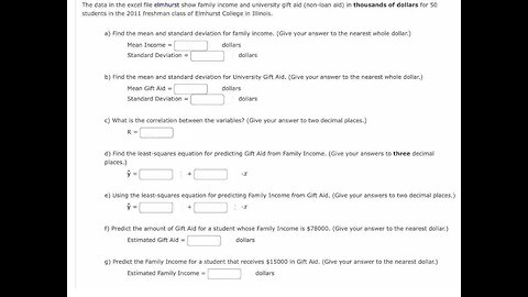
Statistics Help: The data in the excel file elmhurst show family income and university gift aid (non
saxi753
Here is the technique to solve the question related to regressional line and database
#Excel
#RegressionalLine
#Database
#Statistics
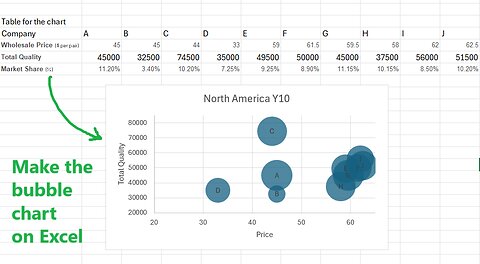
Excel Practice: Business Strategy Game: BSG: How to make the bubble chart for all companies
saxi753
Here is the video to show the step-by-step about Excel and how to make the bubble charts and how to analyze them in here
#BubbleChart
#Techniques
#ExcelPractice
#Answered
#BSG
#BusinessStrategyGame
Finance Help: Consider the mixed streams of cash flows shown in the following table
10 days ago
23
Present value: Mixed streams Consider the mixed streams of cash flows shown in the following table
a. Find the present value of each stream using a 6% discount rate.
b. Compare the calculated present values and discuss them in light of the undiscounted cash flows totaling $70 comma 000 in each case. Is there some discount rate at which the present values of the two streams would be equal?
#FInanceHelp
#AccountingHelp
#Excel
#FutureValue
#Investments
Loading comments...
-
 58:19
58:19
Ben Shapiro
3 hours agoEp. 2131 - Trump and Musk Bring The CHAINSAW
46.3K22 -
 1:12:31
Russell Brand
3 hours agoTrump’s Trade Wars: Power Plays and Global Repercussions – SF531
69.9K36 -
 29:57
29:57
The Finance Hub
1 hour agoBREAKING: DONALD TRUMP JR. JUST DROPPED A MAJOR BOMBSHELL!!!
1.05K6 -
 1:57:48
The Charlie Kirk Show
3 hours agoTrump Gets His Cabinet + Killing the USAID Grift + Why Bud Light Collapsed | Frericks | 2.4.2025
136K39 -
 1:21:47
Simply Bitcoin
3 hours ago $1.56 earnedDid America JUST Change The Bitcoin Nation State Race Forever?! | EP 1175
23.4K3 -
 37:13
37:13
Grant Stinchfield
2 hours ago $4.15 earnedBill Gates is Making the Media Rounds Today to Push the Vax and Stop RFK Jr.
26.7K21 -
 53:03
53:03
TheAlecLaceShow
4 hours agoGuest: Rep. Burgess Owens | Trump Wins with Mexico & Canada | DNC Diversity | The Alec Lace Show
19.4K10 -
 1:00:28
The Dan Bongino Show
5 hours agoTrump’s Most Important Fight To Date (Ep. 2415) - 02/04/2025
693K1.28K -
 59:44
59:44
The Rubin Report
4 hours agoPress Gasps When Shown What USAID Spent Money On
92.7K121 -
 1:15:21
Bare Knuckle Fighting Championship
5 hours agoThe Bare Knuckle Show with Brian Soscia
21.1K3