Premium Only Content

Diaz Marketing - SAM Project 1b Excel Module 01 Creating a Worksheet and a Chart - Step-by-step
Shelly Cashman Excel 365/2021 | Module 1: SAM Project 1b
Diaz Marketing
COMPLETE A BUDGET SUMMARY WORKSHEET
GETTING STARTED
• Save the file SC_EX365_2021_1b_FirstLastName_1.xlsx as SC_EX365_2021_1b_FirstLastName_2.xlsx
o Edit the file name by changing “1” to “2”.
o If you do not see the .xlsx file extension, do not type it. The file extension will be added for you automatically.
• With the file SC_EX365_2021_1b_FirstLastName_2.xlsx open, ensure that your first and last name is displayed in cell B6 of the Documentation worksheet.
o If cell B6 does not display your name, delete the file and download a new copy.
PROJECT STEPS
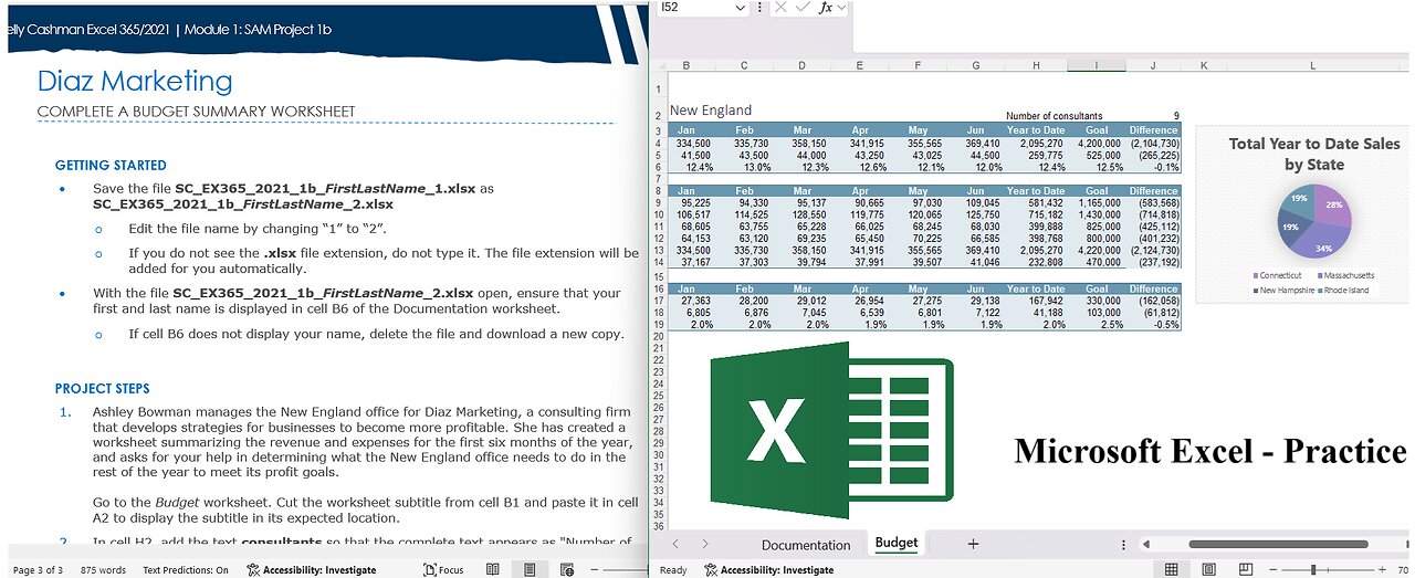
1. Ashley Bowman manages the New England office for Diaz Marketing, a consulting firm that develops strategies for businesses to become more profitable. She has created a worksheet summarizing the revenue and expenses for the first six months of the year, and asks for your help in determining what the New England office needs to do in the rest of the year to meet its profit goals.
Go to the Budget worksheet. Cut the worksheet subtitle from cell B1 and paste it in cell A2 to display the subtitle in its expected location.
2. In cell H2, add the text consultants so that the complete text appears as "Number of consultants" and more clearly identifies the value in cell J2.
3. Enter Feb in cell C3, Mar in cell D3, Apr in cell E3, May in cell F3, and Jun in cell G3.
4. In cell J4, enter a formula that subtracts the value in cell I4 from the value in cell H4 to determine how much revenue the New England office needs to earn from July to December to reach its goal for the year.
5. Ashley wants to calculate the gross margin from January to June and for the year to date. Provide this information as follows:
a. In cell B6, enter a formula that divides the value in cell B5 (the gross profit for January) by the value in cell B4 (the revenue in January).
b. Use the Fill Handle to fill the range C6:H6 with the formula in cell B6 to find the gross margin for February to June and for the year to date.
6. Ashley needs to sum the sales for each New England state for the year to date. Provide this information as follows:
a. In cell H9, enter a formula that uses the SUM function to total the range B9:G9 to calculate the year-to-date sales for Connecticut.
b. Use the Fill Handle to fill the range H10:H12 with the formula in cell H9 to find the year-to-date sales for the other states.
7. In cell B17, enter 27,363 as the general expenses for January.
8. Ashley wants to determine how much revenue each state needs to generate from July to December to reach its target for the year. Enter this information as follows:
a. In cell J9, enter a formula that subtracts the value in cell I9 from the value in cell H9 to find the amount of Connecticut sales Ashley needs to meet the goal.
b. Copy the formula in cell J9, and then paste it in the range J10:J14, pasting the formulas only, to find the differences for the other states, the total, and the revenue per consultant.
9. Ashley is interested in how much revenue the nine consultants each generate on average per month and for the year to date. Find this information as follows:
a. Edit cell B14 to include a formula that divides the value in cell B13 (the total sales for Connecticut in January) by the value in cell J2 (the number of consultants). Don't change the reference to cell J2 that is already there.
b. Fill the range C14:H14 with the formula in cell B14 to determine the average revenue per consultant from February to June and for the year to date.
10. Ashley also needs to calculate the operating margin, which is the ratio of operating profit or loss to revenue and indicates how much the office makes after paying for expenses. Calculate the operating margin as follows:
a. In cell B19, enter a formula that divides the value in cell B18 (the operating profit or loss in January) by the value in cell B4 (the revenue in January).
b. Use the Fill Handle to fill the range C19:H19 with the formula in cell B19 to find the operating margin for February to June and for the year to date.
11. Ashley wants to visualize the total year to date sales separated into states. Insert a chart to provide this visualization as follows:
a. Create a 2-D Pie Chart based on the nonadjacent ranges A8:A12 and H8:H12.
b. Enter Total Year to Date Sales by State as the chart title.
c. Reposition and resize the chart so its upper-left corner is in cell K3 and its bottom-right corner is in cell M17
d. Apply Style 11 to the chart.
12. Hide the gridlines for the Budget worksheet to make it easier to read.
Your workbook should look like the Final Figures on the following pages. Save your changes, close the workbook, and then exit Excel. Follow the directions on the website to submit your completed project.
Final Figure 1: Budget Worksheet
-
 56:15
56:15
Candace Show Podcast
5 hours agoBREAKING: My FIRST Prison Phone Call With Harvey Weinstein | Candace Ep 153
107K65 -
 LIVE
LIVE
megimu32
1 hour agoON THE SUBJECT: The Epstein List & Disney Channel Original Movies Nostalgia!!
184 watching -
 9:06
9:06
Colion Noir
10 hours agoKid With Gun Shoots & Kills 2 Armed Robbers During Home Invasion
16.9K3 -
 54:28
54:28
LFA TV
1 day agoUnjust Man | TRUMPET DAILY 2.27.25 7PM
19.7K2 -
 DVR
DVR
CatfishedOnline
6 hours ago $1.19 earnedGoing Live With Allen Weekly Recap
21.8K -
 20:10
20:10
CartierFamily
7 hours agoAndrew Schulz DESTROYS Charlamagne’s WOKE Meltdown on DOGE & Elon Musk!
36.8K45 -
 1:36:39
Redacted News
5 hours agoBOMBSHELL EPSTEIN SH*T SHOW JUST DROPPED ON WASHINGTON, WHAT IS THIS? | Redacted w Clayton Morris
145K242 -
 2:03:31
Revenge of the Cis
6 hours agoEpisode 1453: Fat & Fit
48.6K8 -
 2:38:12
The White House
7 hours agoPresident Trump Holds a Press Conference with Prime Minister Keir Starmer of the United Kingdom
160K60 -
 1:01:04
In The Litter Box w/ Jewels & Catturd
1 day agoDrain the Swamp! | In the Litter Box w/ Jewels & Catturd – Ep. 751 – 2/27/2025
91.7K35